Research note / Motion planning
How Much Belief Does It Take to Hit the Brakes?
What prediction errors actually matter to a planner?
TL;DR: We usually score a motion prediction by asking how close it came to what actually happened. I wanted to ask something else: did the error make the car do anything differently?
So I built a tiny planner, kept every predicted path fixed, and changed only the probabilities attached to those paths. In 20 controlled cut-in scenes, two equally large probability errors could have completely different outcomes. One did nothing. The other made the planner change its mind.
This started as a small planning-course experiment. I kept getting stuck on a basic question: once a prediction reaches the planner, which errors actually matter?
The easiest way to find out was to strip the problem down until I could see the whole thing.
Three quick definitions before we start:
- the predictor guesses how nearby cars might move;
- the planner decides what our car should do about it;
- ego just means our car.
One important caveat: this experiment shows that the effect exists. It does not tell us how often it happens in real traffic. More on that later.
The question
Say the predictor gives us three possible futures for a nearby car:
- it stays in its lane;
- it makes a mild cut-in;
- it makes an aggressive cut-in.
Our planner has to choose now: maintain speed, slow down, or brake.
That is the whole setup. Three futures. Three responses.
Normally, the paths and their probabilities all change together. If the planner then picks a different action, we do not really know what caused it. Was it the shape of a path? A missing possibility? A confidence score?
So I froze every path and changed only the probabilities.
Would the planner still react? And if two probability estimates were equally wrong, could one matter much more than the other?
Before getting to the experiment, it helps to walk through how motion prediction is usually evaluated. Each step adds something useful. Each also leaves one annoying hole.
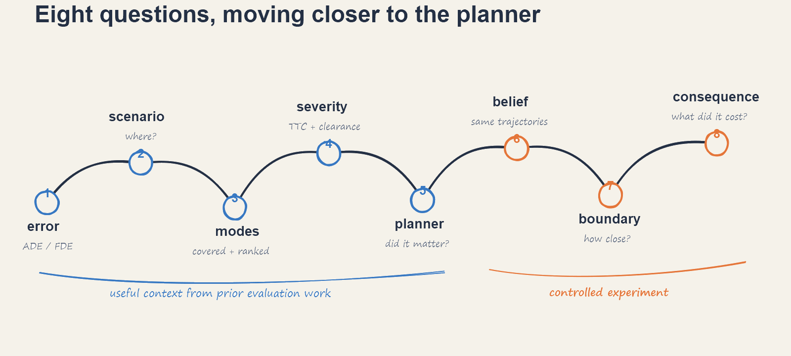
1. How accurate was the prediction?
The obvious place to start is distance.
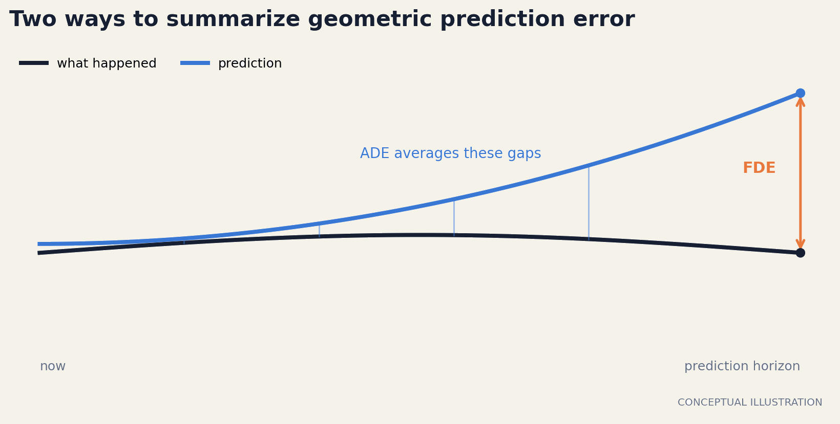
Average displacement error (ADE) measures how far the prediction is from the real path over time. Final displacement error (FDE) only looks at the last point:
$$ FDE = \lVert \hat y_T-y_T \rVert. $$
Simple enough. Did the predicted path land near the real one?
One average can hide difficult maneuvers
One average mixes together a lot of very different driving.
Most cars spend most of their time doing boring, predictable things. They stay in their lane and keep moving. A model can get those scenes right, post a nice average score, and still be bad at merges, turns, lane changes, and cut-ins.
So we can split ADE and FDE by maneuver. This is already much more useful: now we can see where the predictor struggles.
But we are still only measuring geometry. We still do not know whether the model covered the possible futures, whether the miss was dangerous, or whether the planner cared.
2. Did it cover and rank the possible futures?
Driving does not have one obvious future.
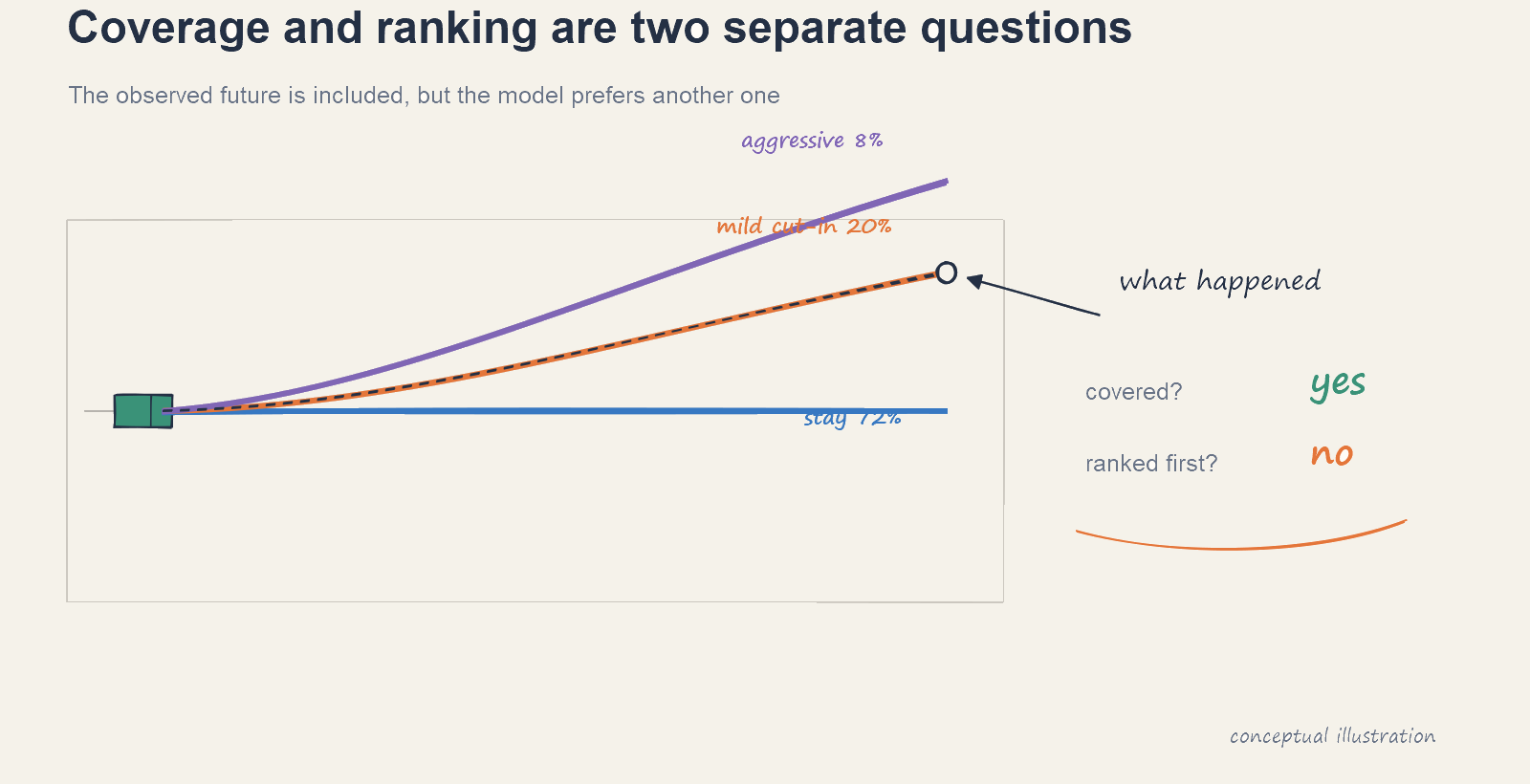
A car near a merge might keep going, merge, yield, or brake. A useful predictor should be able to represent several of these possibilities at once. This is multimodal prediction.
Now we need to ask two things:
- Did the model include the future that actually happened?
- Did it put sensible confidence on each possibility?
minADE and minFDE check whether at least one predicted path came close. Miss rate checks whether all of them missed. Metrics like the Energy Score look at the whole distribution, not just the model's luckiest guess. The Waymo Open Motion Dataset benchmark and models like Motion Transformer use this multimodal view.
Much better. But we still do not know whether a miss was actually dangerous.
3. Was the error dangerous?
This is the part that distance metrics completely flatten.
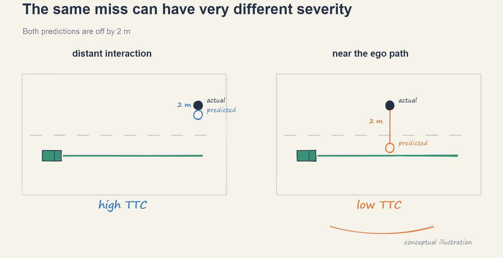
Imagine two predictions that are both wrong by two meters.
In the first scene, the other car is 50 meters away on the other side of an empty road. In the second, it is right next to us and drifting into our lane.
Same FDE. Very different problem.
Things like time to collision (TTC), path overlap, proximity, relative speed, and minimum clearance add the context we were missing. They ask: where did the error happen, and was anyone about to have a really bad day?
4. Did the error matter to the planner?
But even danger is not quite the same as relevance to the planner.
Two scenes can have similar FDE and TTC. In one, both predictions make the car maintain speed. In the other, the prediction changes the action from maintain to brake.
FDE tells us how wrong the path was. TTC tells us how urgent the interaction looked. Neither tells us whether that specific error changed the car's decision.
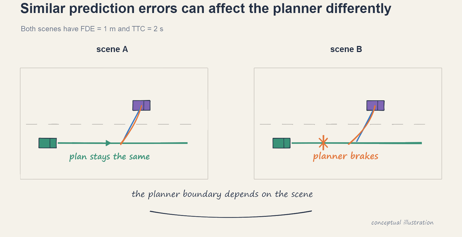
If the planner brakes either way, the error shows up in our metrics but not in the car's behavior. If one prediction says brake and the other says maintain, the error has made it all the way through the stack.
I am definitely not the first person to ask whether prediction metrics match driving quality. Farid et al. connect prediction failures to planning cost. Tran et al. show that better trajectory scores do not always mean better driving. DiffStack trains prediction with the downstream task in mind. CCTR asks whether better confidence calibration helps planning. And Nakamura et al. use regret to find prediction failures that actually hurt the robot downstream.
My question is much narrower.
Keep every possible path exactly where it is. Change only the probabilities. How much belief has to move before the planner changes its mind?
You can also phrase this as a threshold question: how confident does the predictor need to be in a cut-in before the planner hits the brakes?
There is probably no single magic number. A 20% chance of a cut-in might matter a lot when another car is close and moving toward us. The same 20% might mean nothing when there is loads of space. It depends on the scene and on how the planner balances safety, progress, and comfort.
So the experiment has three parts:
- keep the paths fixed and move only their probabilities;
- measure how far the probabilities can move before the action flips;
- check whether that flip actually made the outcome worse.
5. Was it the trajectories or their probabilities?
A multimodal prediction is basically a short list. Each row has one possible path and one probability. Each row is usually called a mode.
- The support is the set of physical paths the model says are possible.
- The belief is the set of probabilities attached to those paths.
Usually both parts change together. Paths move. Modes appear or disappear. Probabilities shift. Good luck figuring out which change the planner reacted to.
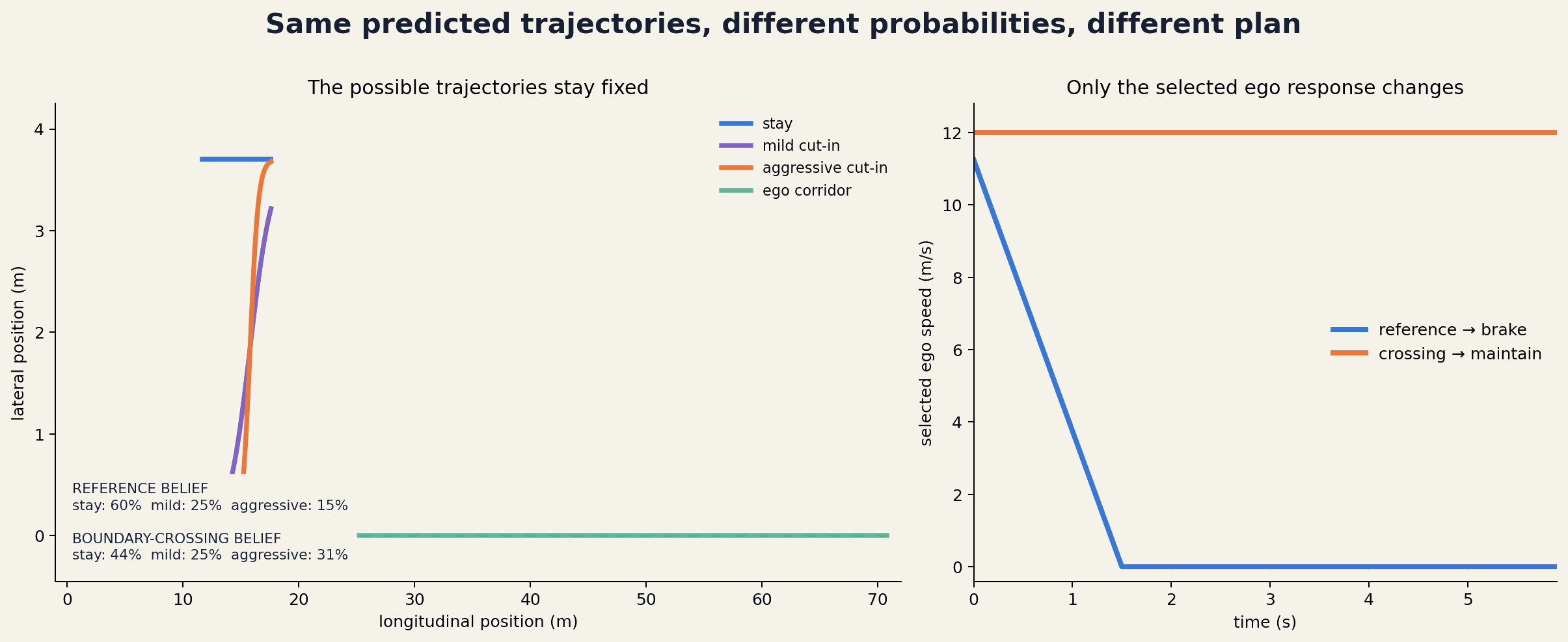
I froze the support instead. No path gets moved, added, removed, or regenerated. I only change the belief.
This means ADE, FDE, coverage, and trajectory diversity literally cannot change. The physical predictions are identical.
In each scene, the other car has three fixed futures: stay in its lane, make a mild cut-in, or make an aggressive cut-in. Ego can maintain speed, slow down, or brake. The planner scores those choices using overlap, clearance, progress, acceleration, and jerk, then picks the cheapest one.
Figure 6 is the whole trick. Same three paths. Different probabilities. That alone changes the ego plan from brake to maintain.
6. How close was the planner to changing its mind?
Now we can ask the question in the title: how much belief has to move before the planner hits the brakes—or stops braking?
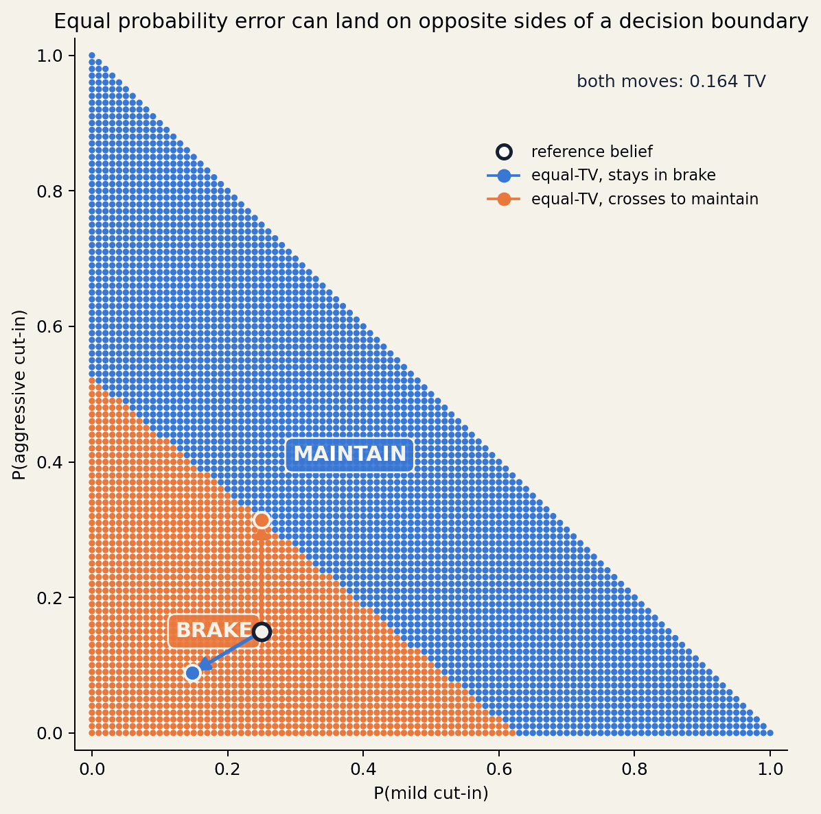
A belief here is just three numbers that add up to one: the probabilities of stay, mild cut-in, and aggressive cut-in. Every possible mix of those numbers fits inside a triangle.
Pick any point in that triangle. The planner uses those probabilities to work out the expected cost of maintaining, slowing down, and braking. Then it picks the cheapest action:
$$ \pi(p)=\arg\min_a J_a(p), \qquad J_a(p)=r_a^\top p. $$
Because this planner is simple and linear, the triangle splits into clean decision regions. One region says maintain. Another says brake. Cross the line and the plan flips.
A real planner would probably produce a much messier boundary. That is fine. The same question still works: how close is the current prediction to making the planner change its mind?
To measure how much probability moved, I used total variation distance:
$$ d_{TV}(p,\tilde p)=\frac{1}{2}\lVert p-\tilde p\rVert_1. $$
Awful name. Simple idea. If I take 0.05 probability from "stay" and give it to "aggressive cut-in," the distance is 0.05. We are measuring probability moved, not meters moved.
I call the smallest change that reaches another decision region $\varepsilon_{flip}$. You can think of it as the planner's margin. Small margin, twitchy decision. Large margin, you have to move a lot of belief before anything changes.
I solved for this distance and also checked it against a dense grid over the triangle.
I tested 20 cut-in settings chosen near transitions between planner actions:
| Quantity | Result |
|---|---|
| Cut-in settings analyzed | 20 / 20 |
| Median distance to nearest competing policy region | 0.1029 TV |
| Scenarios within 0.05 TV of a boundary | 5 / 20 |
| Operational decisions | 18 brake, 2 maintain |
For the median scene, moving 0.1029 of the probability mass was enough to change the plan. Five of the 20 scenes needed no more than 0.05.
That is interesting, but please do not read it as “25% of traffic is near a decision boundary.” I deliberately chose scenes around transitions because I wanted to study the mechanism. This is a microscope, not a traffic survey.
7. Did changing the planner's decision matter?
A plan changing is interesting. It is not automatically bad.
Maybe the new action is safer. Maybe it is less comfortable. Maybe the two choices are basically equivalent. I still needed to check what the change actually cost.
There is also an obvious fairness problem. Comparing one huge error with one tiny error proves very little. So I built pairs with exactly the same amount of probability error. One stays on the same side of the boundary. The other crosses it.
For each scene, I start with one fixed set of reference probabilities, written as $q$. The code calls this the oracle belief. The name is a little grand. It is really just a fixed ruler that lets me compare both errors fairly—not perfect knowledge of a real scene.
I then create two equally large probability errors:
- $p_{in}$ moves the probabilities but stays in the same planner region;
- $p_{cross}$ moves them by the same amount but crosses a boundary.
Their total variation distance from the reference is identical:
$$ d_{TV}(q,p_{in})=d_{TV}(q,p_{cross}). $$
Each altered prediction makes the planner choose an action. I score both actions using the original reference $q$. The prediction changes; the ruler does not.
Any extra cost over the best reference action is oracle regret:
$$ R(p;q)=\mathbb E_q[L(\pi(p),\tau)]-\min_a\mathbb E_q[L(a,\tau)]. $$
In plain English: choose an action using the changed probabilities, then judge that action using the fixed reference probabilities. Zero regret means the changed prediction still led to the best action. Positive regret means it did not.
I also use different weights for choosing the action and judging it. Otherwise the “evaluation” would just repeat the planner's own opinion back to us.
I found a matched pair in all 20 scenes. Every in-region error kept the reference action and had zero regret. Every boundary-crossing error changed the action and had positive regret. The mean gap was 424.52 evaluation-cost units.
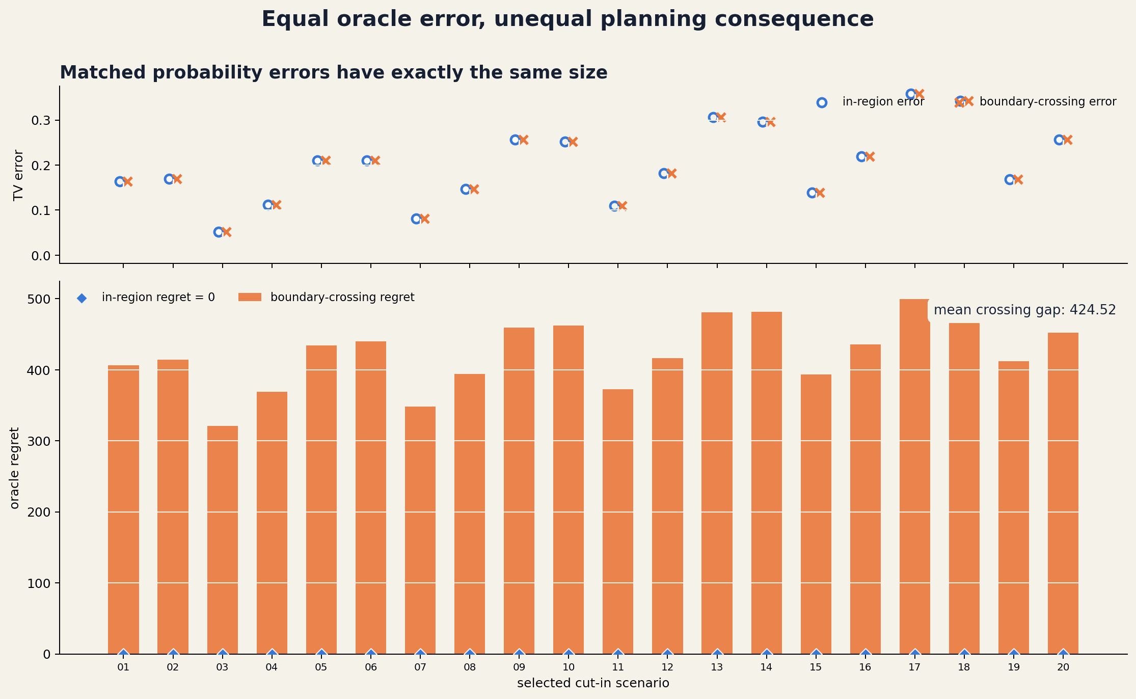
320.99 to 499.27 evaluation-cost units, while explicit blue markers show zero in-region regret.This does not mean “probability errors are bad.” It means error size missed something important in these scenes. Two equally large errors had different consequences because only one crossed the planner's boundary.
Checking nearby planner weights and learned trajectories
The main experiment uses hand-drawn cut-ins and one planner setup. Fair complaint: maybe the result is just a quirk of those choices.
I ran two quick checks. First, I changed how much the planner cares about safety. Then I replaced my hand-drawn paths with outputs from a learned prediction model.
These checks still do not tell us how common the effect is in the real world. They only answer a smaller question: does it immediately disappear when I move away from the base setup?
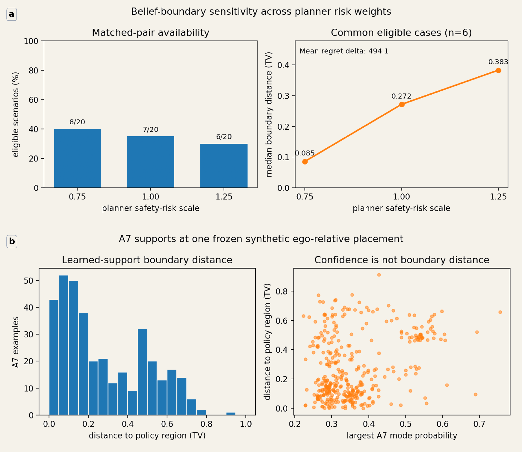
Nearby planner weights
I tried safety-risk weights of 0.75x, 1.00x, and 1.25x while keeping the evaluation rule fixed. The equal-error comparison worked in 8/20, 7/20, and 6/20 scenes.
Six scenes worked under all three settings. In those six, the median boundary distance went from 0.0853 to 0.2719 to 0.3834 TV as the safety weight increased. The mean regret gap stayed at 494.13 evaluation-cost units because the paired cases still switched between the same actions.
I added this common-six comparison after the main experiment, so I see it as a useful sanity check, not a headline result.
Learned trajectory supports
For the second check, I used outputs from a learned motion-prediction model called A7. Each prediction has six paths and six probabilities.
There was one catch: the saved data did not include ego's future. So I placed every prediction at the same synthetic position relative to ego. This makes the scan consistent, but it is a stress test—not a replay of the original driving scenes.
I scanned 500 deterministically selected predictions. For 366 of them, some change in probability could reach a different planner decision. Eight were within 0.01 TV of a boundary, 43 within 0.05, and 95 within 0.10. The planner chose maintain 133 times, slow 143 times, and brake 224 times.
The good news: the boundary idea is not limited to my three hand-drawn paths.
The big caveat: this does not tell me that 8.6% of real Argoverse 2 scenes sit near an important boundary. Without the original ego-agent geometry, I cannot make that claim.
What I take from this
Here is the whole experiment in five lines:
same predicted trajectories
        +
different probabilities
        →
planner boundary crossing
        →
different ego decision
        →
different oracle regret
Geometry tells us where the forecast went. Probability metrics tell us how confidence was split across the possible futures. The planner adds one more question: did the error land somewhere that changed the decision?
I think distance to a planner boundary could be a useful diagnostic beside ADE, FDE, coverage, and calibration. A small error can cross a nearby boundary. A much larger error can stay inside the same region and change nothing.
This is still a deliberately tiny experiment: synthetic cut-ins, one nearby car, and a planner that mostly chooses between maintain and brake. (slow never wins in the base suite.) Models like Scene Transformer and FJMP model joint futures for several agents. The boundary idea might carry over, but interactions between agents could make it behave very differently.
Also, the cost numbers here are not collision probabilities or units of real-world harm. They only let us compare the paired cases inside this experiment.
The mechanism is real. How often it matters in traffic is still an open question.
What I would do next
The obvious next step is to put the learned predictions back into their real scenes.
I would restore the original ego and agent geometry for the saved A7 records, keep every predicted path in its native scene, and run the same analysis again. Then we could finally ask how often real forecasts sit near a boundary that actually matters.
Reproducing it
Everything is deterministic. The code uses NumPy and a small expected-cost planner. A constrained linear program finds the nearest competing decision region, and a dense grid checks the answer.
The repository has frozen configs for the configs/belief_planning_blog.yaml, the configs/belief_planning_balanced_sweep.yaml, and the configs/belief_planning_a7_scan.yaml. The idea3-assets/manifest.json records the checksums and where every figure came from.
If you work on prediction or planning, I would genuinely love to know where this framing breaks. Would you monitor distance to a planner boundary? Or does the whole idea get too unstable once the planner becomes realistic?
References
- Ettinger et al. Large Scale Interactive Motion Forecasting for Autonomous Driving: The Waymo Open Motion Dataset. ICCV, 2021.
- Shi et al. Motion Transformer with Global Intention Localization and Local Movement Refinement. NeurIPS, 2022.
- Farid et al. Task-Relevant Failure Detection for Trajectory Predictors in Autonomous Vehicles. CoRL 2022, published 2023.
- Karkus et al. DiffStack: A Differentiable and Modular Control Stack for Autonomous Vehicles. CoRL, 2022.
- Tran et al. What Truly Matters in Trajectory Prediction for Autonomous Driving?. NeurIPS, 2023.
- Cao et al. CCTR: Calibrating Trajectory Prediction for Uncertainty-Aware Motion Planning in Autonomous Driving. AAAI, 2024.
- Shahroudi et al. Evaluation of Trajectory Distribution Predictions with Energy Score. ICML, 2024.
- Nakamura et al. Not All Errors Are Made Equal: A Regret Metric for Detecting System-level Trajectory Prediction Failures. CoRL, 2024; published 2025.
- Da et al. Measuring What Matters: Scenario-Driven Evaluation for Trajectory Predictors in Autonomous Driving. arXiv preprint, 2025.
- Chakraborty et al. Safety Evaluation of Motion Plans Using Trajectory Predictors as Forward Reachable Set Estimators. arXiv preprint, 2025.
- Ngiam et al. Scene Transformer: A Unified Architecture for Predicting Multiple Agent Trajectories. ICLR, 2022.
- Rowe et al. FJMP: Factorized Joint Multi-Agent Motion Prediction Over Learned Directed Acyclic Interaction Graphs. CVPR, 2023.